MASTERING LINEAR REGRESSION: COMPLETE GUIDE TO INTERPRETATION & DIAGNOSTICS

Introduction
Linear regression is the workhorse of engineering analysis predicting material strength from temperature, modeling system performance, relating quality metrics to process parameters. Yet most engineers use regression without understanding what the numbers mean or whether the model is valid. An R² of 0.85 sounds good, but if residuals show a funnel pattern (heteroscedasticity), your standard errors are wrong. A regression coefficient might be statistically significant but practically meaningless. This guide teaches you how to interpret regression output and validate assumptions before trusting predictions.
Paraphrasing-tool.ai Reviews, Alternatives, Pricing, & Offerings in 2025
Linear Regression Fundamentals
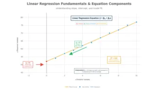
Linear Regression Fundamentals: Equation, Components, and Interpretation
The Regression Equation: ŷ = β₀ + β₁x
ŷ (y-hat): Predicted value of the dependent variable
β₀ (intercept): Y-value when x = 0 (where line crosses y-axis)
β₁ (slope): Change in y for each 1-unit increase in x
x: Independent variable (predictor)
Interpreting Coefficients
Intercept (β₀): Often lacks practical meaning. If x = 0 is outside your data range, the intercept is just a mathematical anchor, not interpretable as a real prediction.
Slope (β₁): THIS is what matters. β₁ = 2.5 means “for each 1-unit increase in x, y increases by 2.5 units on average, holding all else constant.”
Statistical significance of β₁:
- Test using t-statistic: t = β₁ / SE(β₁)
- Compare p-value to α (typically 0.05)
- Small p-value (p < 0.05) means β₁ significantly different from zero
- ≠ Large effect size; statistical significance ≠ practical significance
R² and Adjusted R²
R² (coefficient of determination):
- Measures proportion of y-variance explained by x
- 0 ≤ R² ≤ 1 (0% to 100%)
- R² = 0.85 means x explains 85% of y’s variation; 15% unexplained
- Interpretation caveat: High R² doesn’t mean causation; low R² doesn’t mean model is useless
Adjusted R²:
- Penalizes adding predictors that don’t improve model
- Always ≤ R² (can be negative)
- Preferred for multiple regression with many variables
- Formula: Adjusted R² = 1 – [(1-R²) × (n-1)/(n-k-1)]
- Where n = sample size, k = number of predictors
When R² is low but model is still useful:
- If you’re making predictions in high-variance domains (e.g., stock prices), even R² = 0.30 might be valuable
- Context matters: Chemistry R² = 0.95; ecology R² = 0.40 is acceptable
Best AI Humanizer Tools for Essays
Assumption Checking & Diagnostics
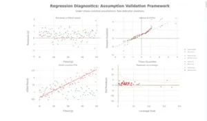
4-Plot Diagnostic Framework: Assessing Linear Regression Assumptions
Regression validity depends on four critical assumptions. Violating them leads to unreliable coefficient estimates, biased standard errors, and invalid hypothesis tests.
Assumption 1: Linearity
What it means: Relationship between x and y is linear (straight line, not curved)
How to check:
- Scatter plot of x vs. y: Points should follow roughly straight pattern
- Residuals vs. Fitted plot: No curved pattern (should be random scatter)
- If curved: Linear model is misspecified
If violated:
- Transformation: Log(y) or √x might linearize relationship
- Polynomial regression: Add x² term (quadratic)
- Non-linear regression: Use exponential or power law models
Assumption 2: Independence
What it means: Observations are independent; no autocorrelation (residuals not related to each other)
How to check:
- Data collection method (Was sampling random? Or sequential/clustered?)
- Durbin-Watson test (for time-series data)
- Plot residuals vs. observation order: Should be random pattern
If violated: (Common in time-series, spatial data)
- Use time-series models (ARIMA)
- Add lag variables
- Use mixed effects models accounting for clustering
Assumption 3: Homoscedasticity (Constant Variance)
What it means: Residuals have equal variance across all x values (not heteroscedastic)
How to check:
- Residuals vs. Fitted plot: Should show random scatter with constant spread
- Good: Points scattered evenly around zero
- Bad: Funnel pattern (spread increases/decreases with fitted values)
- Scale-Location plot: Shows √|standardized residuals| vs fitted values
- Good: Horizontal trend line
- Bad: Upward or downward trend
Statistical test: Breusch-Pagan test
- Small p-value (p < 0.05) indicates heteroscedasticity
If violated:
- Weighted least squares regression (weight by 1/variance)
- Variance-stabilizing transformation: Log(y), √y, or 1/y
- Robust standard errors (Huber-White) preserve estimates but correct SE
Rephrasy.ai Review 2025: The Game-Changing AI Humanizer That Actually Delivers
Assumption 4: Normality of Residuals
What it means: Residuals follow normal distribution with mean = 0
How to check:
- Normal Q-Q plot: Points should follow diagonal line
- Good: Close to straight line throughout
- Bad: S-shaped curve (heavy tails), systematic deviation at ends
- Histogram of residuals: Should be bell-shaped
- Shapiro-Wilk test: p < 0.05 indicates non-normality
Visual interpretation patterns:
- Upper tail deviation: Right skew or outliers
- Lower tail deviation: Left skew or outliers
- S-shaped pattern: Heavy tails (more extreme values than normal)
If violated:
- For large samples: Central Limit Theorem makes this less critical
- Box-Cox transformation can normalize residuals
- Robust regression (reduce outlier influence)
- Non-parametric regression alternatives
Identifying Influential Points & Outliers

Multicollinearity Detection: VIF Scale, Symptoms, and Remedial Actions
Not all outliers affect regression equally. Understanding leverage, residuals, and influence is critical.
Three Types of Unusual Points
Outlier: Unusual y-value (large residual) but x-value in normal range
- Issue: Violates normality assumption
- Influence: Low if near center of x-distribution
- Fix: Transform data, check for data entry errors, robust regression
Leverage Point: Unusual x-value (far from x-mean) but y follows regression line
- Issue: Point follows pattern but far from others
- Influence: CAN inflate R² and statistical significance even though coefficient unchanged
- Fix: Usually keep (if valid); note in report
Influential Point: Both unusual x and large residual; pulls regression line
- Issue: Significantly changes slope or intercept if removed
- Influence: CRITICAL—coefficient estimates unreliable
- Fix: Investigate data quality; consider robust regression; report sensitivity
Detecting Influential Points: Cook’s Distance
Cook’s Distance formula: D_i = (Residual_i)² / (p × MSE) × Leverage_i
Interpretation:
- D < 0.5: Not influential
- 0.5 < D < 1.0: Somewhat influential; investigate
- D > 1.0: Highly influential; likely problematic
- Rule of thumb: D > 4/n indicates influential outlier
Example:
- Sample size n = 50
- Threshold: 4/50 = 0.08
- Points with D > 0.08 are influential outliers
How to handle:
- Verify data quality: Is it a data entry error? Measurement error?
- Understand context: Is it a legitimate extreme value?
- Sensitivity analysis: Refit without point; compare coefficients
- Report: Always mention influential points in analysis
- Robust regression: Reduces influence of outliers
Otter.ai Reviews, Best Alternatives, Pricing, & Offerings in 2025
Engineering Applications
Application 1: Predicting Material Strength from Temperature
Scenario:
Steel tensile strength (MPa) predicted from temperature (°C)
Data: 22 measurements from -320°F to +80°F
Regression model: Strength = β₀ + β₁ × Temperature
Result from NIST data:
- As temperature increases, steel strength decreases
- Linear relationship explains 94% of variation (R² = 0.94)
- Coefficients quantify strength loss per degree
- Used for structural safety analysis in fire conditions
Diagnostics to check:
- Residuals vs. Fitted: Constant variance across temp range?
- Q-Q plot: Residuals normally distributed?
- Influential points: Are extreme temps unduly influential?
- Prediction intervals: How wide for future measurements?
Application 2: Quality Control—Relating Defect Rate to Process Temperature
Scenario: Electronics manufacturing
- Response: Defect rate (%)
- Predictor: Reflow oven temperature (°C)
Model: Defect_Rate = β₀ + β₁ × Oven_Temp
Expected pattern:
- Temperature too low → high defects (cold solder joints)
- Temperature optimal → low defects
- Temperature too high → high defects (component damage)
- Non-linear U-shaped pattern
Regression issue: Simple linear regression won’t fit U-shape!
Solution: Add quadratic term
- Model: Defect = β₀ + β₁ × Temp + β₂ × Temp²
- Now captures optimal temperature and tail-off effects
Engineering insight: Check residuals vs. fitted; if curved pattern, polynomial needed
Application 3: System Performance Modeling
Scenario: Server processing time vs. CPU load
Linear regression: Processing_Time = β₀ + β₁ × CPU_Load
Typical result: As CPU load increases, processing time increases linearly (slope positive)
Multicollinearity issue: If you have multiple CPU cores, memory usage, disk I/O as predictors
- These are often correlated with each other
- Use VIF to detect: VIF > 10 for any predictor?
- Solution: Remove less important correlated predictor or use ridge regression
AllMath Review: How Effective Is Its AI Math Solver?
Multiple Regression & Multicollinearity

Multicollinearity Detection: VIF Scale, Symptoms, and Remedial Actions
What is Multicollinearity?
Definition: When two or more predictor variables are highly correlated with each other
Why it’s a problem:
- Inflates standard errors of coefficients
- Makes estimates unstable (small data change → large coefficient change)
- Coefficients become hard to interpret
- Hypothesis tests become unreliable (wide confidence intervals)
Detecting Multicollinearity
Method 1: Correlation Matrix
- Calculate pairwise correlations between predictors
- Correlation > 0.8 suggests potential multicollinearity
- Limitation: Only detects pairwise; misses multi-way correlations
Method 2: Variance Inflation Factor (VIF)
- Calculated for EACH predictor
- VIF_j = 1 / (1 – R_j²)
- Where R_j² is R² from regressing predictor j on all other predictors
VIF interpretation:
- VIF = 1: No multicollinearity (ideal)
- VIF 1-4: Low; usually acceptable
- VIF 4-10: Moderate; investigate
- VIF > 10: Severe; take action
Example:
If VIF_Weight = 8.42, variance of weight coefficient is 8.42 times inflated due to correlation with other predictors
Fixing Multicollinearity
Option 1: Remove Variable (Simplest)
- Drop the less important correlated predictor
- Trade-off: Lose information, but gain interpretability
- Use case: When one variable is clearly secondary
Option 2: Ridge Regression
- Shrinks coefficients toward zero
- Reduces variance at cost of bias
- Still includes all predictors
- Use case: Want to keep all variables but stabilize estimates
Option 3: Lasso Regression
- Shrinks some coefficients exactly to zero (variable selection)
- Simultaneously selects variables and reduces multicollinearity
- Use case: Many predictors; want automatic selection
Option 4: Principal Component Analysis (PCA)
- Creates new uncorrelated variables (principal components)
- Trades interpretability for reduced multicollinearity
- Use case: Very high-dimensional data with many correlated variables
Software Walkthroughs
Excel
text
=LINEST(y_range, x_range, TRUE, TRUE)
Returns: slope, intercept, slopes_SE, intercept_SE, R², std_error, F, dof, SS_reg, SS_residual
Manual R² calculation:
=1 – SUMSQ(residuals)/SUMSQ(y – AVERAGE(y))
Prediction with confidence interval:
Point estimate: β₀ + β₁ × x_new
SE(pred) = √[MSE × (1 + 1/n + (x_new – x̄)²/Σ(x-x̄)²)]
Interval: Estimate ± t_critical × SE(pred)
R
r
# Fit linear regression
model <- lm(y ~ x, data = mydata)
# Summary statistics
summary(model) # Coefficients, p-values, R², F-test
confint(model) # 95% CI for coefficients
# Diagnostics
plot(model) # 4-panel diagnostic plots
par(mfrow=c(2,2))
plot(model)
# Specific tests
shapiro.test(residuals(model)) # Normality test
lmtest::bptest(model) # Heteroscedasticity test (Breusch-Pagan)
car::vif(model) # VIF for multicollinearity
# Influence diagnostics
cooks.distance(model) # Cook’s distance
hatvalues(model) # Leverage values
rstudent(model) # Studentized residuals
# Multiple regression with interactions
model2 <- lm(y ~ x1 + x2 + x1:x2, data = mydata)
# Ridge regression (for multicollinearity)
library(glmnet)
ridge_model <- glmnet(x_matrix, y, alpha=0)
Python (scikit-learn, statsmodels)
python
# Using statsmodels (more diagnostic output)
import statsmodels.api as sm
import numpy as np
# Add constant for intercept
X = sm.add_constant(X)
model = sm.OLS(y, X).fit()
# Summary
print(model.summary()) # Full regression summary
# Diagnostics
from statsmodels.graphics.gofplots import ProbPlot
import matplotlib.pyplot as plt
fig, axes = plt.subplots(2, 2)
fig = sm.graphics.plot_partregress_grid(model, fig=fig)
plt.show()
# VIF
from statsmodels.stats.outliers_influence import variance_inflation_factor
vif = [variance_inflation_factor(X.values, i) for i in range(X.shape[1])]
# Cook’s distance
from statsmodels.graphics.gofplots import OLSInfluencePlots
influence_plot(model)
# Using scikit-learn (simpler)
from sklearn.linear_model import LinearRegression
model_sk = LinearRegression().fit(X, y)
r2 = model_sk.score(X, y)
SPSS
text
Analyze → Regression → Linear
– Dependent: y variable
– Independent(s): x variable(s)
– Statistics: Estimates, Model Fit, Descriptives, Diagnostics
– Plots: Residuals plots (Standardized vs. Predicted)
Output includes:
– ANOVA table (F-test for overall significance)
– Coefficients table (β, SE, t, p-value)
– Diagnostics (R², Durbin-Watson)
Tutoring for Struggling Students 2026: How to Help Without Harm
Common Mistakes & How to Avoid Them
Mistake 1: Correlation ≠ Causation
Example: Ice cream sales correlate with drowning deaths.
- Correlation: 0.92 (very strong)
- Causation: Neither causes the other; both caused by summer temperature
In regression: A significant β₁ doesn’t prove x causes y
- Could be reversed causation
- Could be confounding variable
- Could be coincidence with spurious association
How to avoid:
- Use controlled experiments, not observational data
- Report correlations, not causal claims
- Acknowledge limitations
Mistake 2: Using Regression Outside Data Range (Extrapolation)
Example: Temperature range in data: 0–100°C
- Using model to predict strength at 500°C
- Relationship may become non-linear outside observed range
- Prediction interval explodes as x moves away from data mean
How to avoid:
- Note prediction intervals: wider at extremes
- Don’t extrapolate beyond ±10% of observed x range
- Add warning: “Predictions outside observed range unreliable”
Mistake 3: Ignoring Multicollinearity
Example: Predicting price with Height AND Weight (highly correlated)
- Both individually significant (p < 0.05)
- But standard errors so large that individual slopes unreliable
- Coefficients flip sign if you drop one variable
How to avoid:
- Always calculate VIF: car::vif(model) in R
- If VIF > 10: Remove variable or use ridge regression
- Report VIF in analysis
Mistake 4: Assuming Residuals Are Normal
Example: Regression on percentage data (0–100%)
- Residuals tend to be non-normal (bounded)
- Normal regression inappropriate; use logistic regression instead
How to avoid:
- Always check Q-Q plot
- Run Shapiro-Wilk test
- If non-normal: Transform (log, sqrt) or use robust regression
Mistake 5: Ignoring Heteroscedasticity
Example: Predicting error rate by part size
- Small parts: measurement error ±1%
- Large parts: measurement error ±5%
- Variance increases with part size (heteroscedasticity)
- Standard errors underestimated
How to avoid:
- Plot residuals vs. fitted values
- Breusch-Pagan test for heteroscedasticity
- If heteroscedastic: Weighted least squares or variance transformation
Textero Review: A Tool That Changes the Approach to Learning
Practice Problems with Solutions
Problem 1:
A manufacturer collects 30 samples relating oven temperature (°C) to defect rate (%).
Data summary: x̄ = 200, s_x = 15, ȳ = 5.2, s_y = 2.1, r = -0.82
Calculate the regression equation.
Solution:
β₁ = r × (s_y / s_x) = -0.82 × (2.1 / 15) = -0.1148
β₀ = ȳ – β₁ × x̄ = 5.2 – (-0.1148) × 200 = 28.16
Regression equation: Defect_Rate = 28.16 – 0.1148 × Temperature
Interpretation: Each 1°C increase in temperature reduces defect rate by 0.115% on average.
Problem 2:
A regression model shows:
- R² = 0.88
- Residuals vs. Fitted plot shows funnel pattern (increasing spread)
- Normal Q-Q plot shows S-shaped curve
What problems exist? How to fix?
Solution:
Problems identified:
- Heteroscedasticity: Funnel pattern indicates non-constant variance
- Non-normality: S-shaped Q-Q suggests heavy tails or skew
Fixes:
- Apply weighted least squares with weights = 1/variance
- Try variance-stabilizing transformation: Log(y) or √y
- Use robust standard errors (preserves estimates, corrects SE)
- Check for outliers pulling tails
Key Takeaways
- Regression equation: ŷ = β₀ + β₁x; interpret β₁ as “y changes β₁ units per 1-unit x increase”
- R² measures fit: 85% means x explains 85% of y variation; doesn’t imply causation
- Four key assumptions: Linearity, independence, homoscedasticity, normality
- Always check diagnostics: Residuals plots + Q-Q plot before trusting model
- Multicollinearity inflates uncertainty: VIF > 10 is red flag; remove variable or use ridge regression
- Influential outliers matter: Cook’s D > 1 indicates points pulling regression line
- Context determines significance: Low R² acceptable in high-variance domains; practical ≠ statistical significance
- Software validates assumptions: R plots, Python statsmodels, SPSS diagnostics all provide necessary checks
Need help with your regression project? [Explore statistics tutoring at MyEngineeringBuddy—Expert guidance for engineering students and professionals]
******************************
This article provides general educational guidance only. It is NOT official exam policy, professional academic advice, or guaranteed results. Always verify information with your school, official exam boards (College Board, Cambridge, IB), or qualified professionals before making decisions. Read Full Policies & Disclaimer , Contact Us To Report An Error