The Quantum Shift in Allocation: How LSTM Models Strengthen Portfolio Risk and Returns

Where MPT Breaks Down in Practice

The core idea behind MVO is simple: estimate expected returns, compute a covariance matrix, and solve for weights that maximize return for a given level of risk. The issue is not the math but the assumptions. Several limitations show up immediately in real data.

Linear Covariance Assumption

Financial correlations are not stable. Equity and credit correlations rise during drawdowns, while FX and rates may behave differently across regimes. MVO treats correlations as linear and fixed, which means it often understates risk during expansion periods and overstates diversification benefits during stress.

Temporal Instability

The covariance matrix is only a snapshot. If markets transition from low to high volatility, the optimizer has no awareness of recent changes. It does not “remember” the conditions that led to the current state. As Dr Thomas Starke, faculty for QuantInsti’s Executive Programme in Algorithmic Trading, often notes, ignoring the path of returns removes valuable information that could strengthen allocation decisions.

Estimation Error

Even with large datasets, covariance matrices are notoriously noisy. A small change in the estimated inputs leads to disproportionate changes in weight allocations.

To understand why modern markets challenge traditional theory, let’s compare the static approach of MPT with the dynamic nature of LSTMs. The following breakdown highlights the fundamental shift in how risk is perceived.

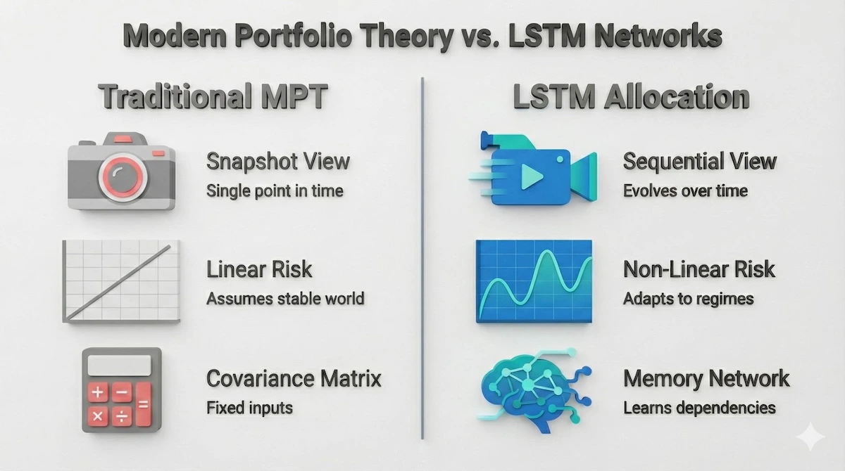
Static models like MPT take a snapshot of risk, while LSTMs analyze the entire movie of market behavior.

As the visual demonstrates, moving from a static snapshot to a sequential view allows for better risk adaptation in changing market environments.

This instability is one of the main reasons professional quants often regularize or replace MVO entirely.These issues compound in environments where relationships shift quickly — which is now the norm rather than the exception.

LSTMs Provide Temporal Awareness and Non-linear Insight

LSTMs are a subclass of recurrent neural networks designed to work with sequences. What makes them useful in finance is not magic but structure: they store information over longer periods, allowing them to capture how returns, volatility, and correlations evolve.

LSTMs are not a direct replacement for an optimizer. Instead, they enhance the upstream information feeding into the allocation process. Two areas are particularly important.

1. Forecasting Inputs That Are Hard to Model Linearly

In many portfolio systems, expected returns come from predictive signals. An LSTM can refine these signals by learning:

• shifts in volatility regimes
• correlation breakdowns
• momentum decay and reacceleration
• macro-driven changes in risk premia

Even modest improvements in forecasting translate into better weight decisions downstream. This integration of predicted insights into position sizing is one of the reasons machine learning in portfolio management is gaining traction among quants.

This integration isn’t about replacing the optimizer, but enhancing the fuel it runs on. The flowchart below illustrates exactly how the LSTM engine processes data before it ever reaches the allocation stage.

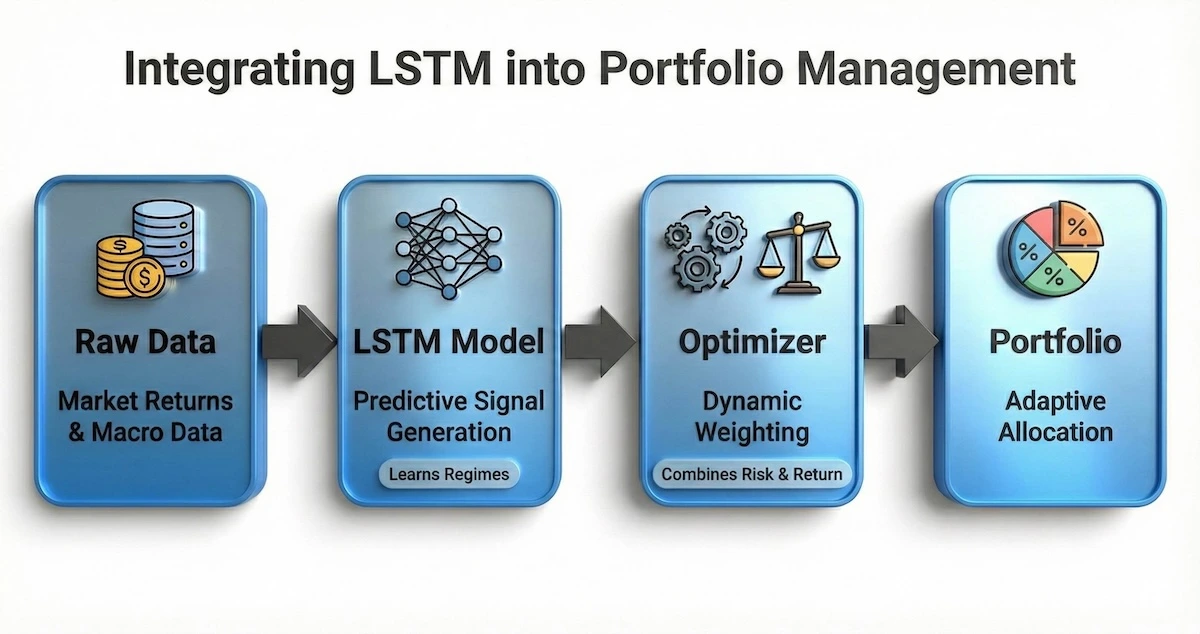
LSTMs don’t replace the optimizer; they upgrade the fuel (data signals) that powers the engine.

By refining the inputs first—cleaning the signal before the noise enters the optimizer—the final weight allocation becomes far more robust.

2. Learning Non-linear Risk Structures

Risk is rarely linear. Correlations spike during crises, and volatility clustering can produce long memory effects. LSTMs can model these effects because they learn patterns that unfold over time instead of reducing everything to a single covariance estimate.

Dr Starke’s research repeatedly shows that when temporal dynamics and predictive signals are combined before optimization, out-of-sample results often improve. These improvements are not guaranteed but tend to appear when models are trained with disciplined validation methods and realistic assumptions.

Why LSTMs Often Outperform MVO in Out-of-Sample Testing

Several techniques help explain why LSTM-based systems can outperform classical allocation.

Hierarchical Risk Parity and HERC

Machine learning-driven allocators like HRP and HERC inherently reduce estimation error by clustering assets and allocating risk more evenly. They remain more stable when covariance structures change suddenly. These methods consistently outperform equal weighting and inverse volatility allocation in many empirical studies.

Integration of Dynamic Inputs

The output of an LSTM does not need to be a direct weight. It can be a volatility forecast, a regime indicator, a correlation estimate, or even a probability of a drawdown event. Feeding dynamic estimates into an optimizer often produces more robust allocations.

Awareness of Regime Shifts

A key advantage of LSTMs is their ability to recognize when the market mood changes, known as a regime shift. This chart demonstrates how non-linear models react to volatility spikes that linear models often miss.

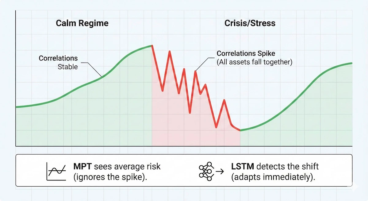
During market stress, correlations spike. LSTMs detect this “regime shift,” whereas traditional models simply see average noise.

Notice how the model detects the ‘stress regime’ (in red) early, allowing for defensive positioning before the worst impacts of the drawdown hit.

Because LSTMs process sequences, they naturally adjust when markets move from calm to stressed conditions. A classical optimizer has no such memory unless explicitly engineered into the model.

Avoiding Common Pitfalls When Using LSTMs

LSTMs can perform well, but they also introduce real challenges.

Overfitting to History

Financial time series have low signal-to-noise ratios, making overfitting a serious risk. Walk-forward optimization is essential because it forces the model to train only on past data and validate on unseen future segments. This process is emphasized heavily in QuantInsti’s AI portfolio management course because it prevents the illusion of perfect equity curves that never survive live trading.

To prevent your model from memorizing the past, you must use a rigorous testing framework. The diagram below outlines the ‘Walk-Forward’ validation method, which is essential for ensuring your results are real.

To avoid overfitting, LSTMs must be tested using a “sliding window” that strictly separates past training data from future validation data.

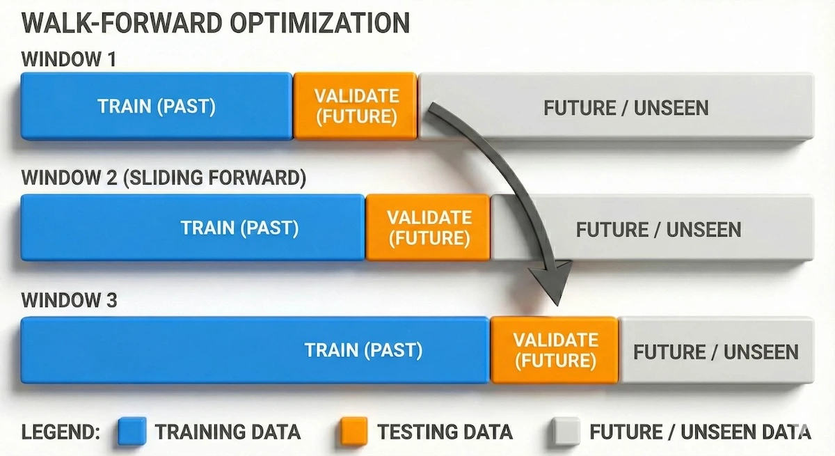
By constantly sliding the training window forward, we ensure the model is always tested on unseen data, simulating the reality of live trading.

Data Quality and Feature Engineering

Clean and relevant data matters more than network size. Quants must handle missing values and outliers carefully, normalize inputs appropriately, and create features that genuinely add signal. As Raimondo Marino’s research highlighted, preprocessing directly influences the performance of every downstream step. Advanced quants often borrow techniques from Lopez de Prado, such as fractional differentiation, to achieve partial stationarity without discarding valuable information.

Hyperparameter Tuning

LSTMs have many tunable components. Grid search is inefficient and often computationally unrealistic, so practitioners rely on smarter search methods. These tuning processes typically require thousands of simulations, and the optimization must be repeated across multiple walk-forward windows to ensure robustness.

Bringing It All Together

When integrated properly, LSTMs and modern optimization techniques create a more adaptive allocation framework. This does not replace financial intuition; instead, it builds on it. Quants can combine predictive signals, dynamic volatility estimates, and stability-driven allocators like HRP to build portfolios that respond more naturally to changing conditions.

For hands-on code, example notebooks, and practical walkthroughs that mirror the workflows discussed here, check My Engineering Buddy website.

Those resources — including LSTM pipelines, walk-forward scripts, and HRP implementations — are designed to help you translate theory into production-ready experiments.

The real value lies in the improvement of out-of-sample performance. While MVO often struggles once the market environment shifts, systems enriched with sequential learning and non-linear modeling tend to hold up better.

For professionals exploring this space, QuantInsti’s AI portfolio management course offers a structured environment to study how LSTMs, walk-forward testing, and modern allocation methods work in practice.

Conclusion

Markets have evolved beyond the static assumptions that shaped early portfolio theory. While MVO remains an important foundation, its limitations are clear. LSTMs offer a way to incorporate temporal patterns, non-linear relationships, and predictive signals directly into the allocation pipeline. When combined with rigorous testing and responsible data engineering, they provide a practical path toward more resilient and adaptive portfolio construction.

For quants building the next generation of strategies, mastering these tools is no longer optional. It is part of the natural evolution of machine learning in portfolio management and a necessary step toward achieving robust, sustainable alpha in a world where efficiency is rising and regimes shift faster than ever.